|
If a partially
sighted person is to use this device in his or her everyday life, it must
be portable and usable anywhere. Moreover,
it would be beneficial if the system were not just thought of as a tool
that helped people to see better, but as an extension of a person's visual
apparatus, always in use. This
would require a seamless integration with the user and is an example of
interactional constancy.
To achieve this
interactional constancy, a computer must be worn by the user at all times.
The ideal device for this is a wearable computer running the Linux
Debian/GNU operating system. Additionally,
the display should show what the user can see without a camera in the way.
This is accomplished with the use of the EyeTap invention.
The EyeTap
invention mediates reality within a portion of the field of view. This is
done by interposing a double-sided mirror between the eye and a given
scene. The mirror reflects
incoming light to a camera, which is located an inch or so to the side. The camera then sends the image to the computer, which
reconstructs it using a heads-up display on the other side of the mirror.
The mirror is
positioned at a 45 degree angle so that the incoming light is collinear
with the outgoing rays. In effect, the invention modifies real light into
virtual light, so that the person has the illusion of 'seeing' through the
mirror.
The camera itself
is a Connectix QuickCam digital apparatus that captures video roughly once
a second, and sends it to the parallel port of the computer.
The Viewfinder program is the software skeleton for
this project. It was
developed by Professor Steve Mann in an effort to provide real-time video
that could be displayed by a wearable computer.
The program itself is the software interface between
the QuickCam digital camera, the Linux operating system, and the video
hardware that actually displays video.
The operation of the Viewfinder program is as
follows:
·
Allocate buffer memory for a frame.
·
Read data into the buffer from the digital camera.
·
Copy the buffer to the video hardware.
The goal of this project is to create a visual
enhancement system for the partially sighted.
The implementation is a modified version of Professor Mann's
Viewfinder program. What was
done over the course of the project was to modify the Viewfinder program
so that it would intercept images captured from the digital camera,
perform image processing on them, and output the new image to the video
hardware.
The image processing that is done on the image is
called edge detection, which will be explained in detail in the next
section.
The basic algorithm for edge detection is to take x-
and y- derivatives of an image and combine them using a Pythagorean
operator.
The new operation of the Viewfinder program is as
follows:
·
Allocate buffer memory for a frame and its corresponding
edge map.
·
Read data into the buffer from the digital camera.
·
Take the x- and y- derivatives of the image using a
2-dimensional convolutional kernel.
·
Combine the x- and y- derivative images pixel-by-pixel using
a Pythagorean operator.
·
Perform adaptive dynamic range correction on the resulting
image.
·
Output the image to the video hardware.
Edge Detection is
an imaging technique that analyses a picture for high-contrast areas and
outputs a map of these edges in black and white.
The purpose of edge detection in this context is to remove
extraneous detail from view, leaving only object details present.
This will enable a visually impaired person to 'see' the object
without having to distinguish between colors, textures, and so on.
An excellent example of this is an edge-detected version of the
Linux Penguin.

Linux Logo |
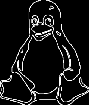
Edge-detected Linux Logo |
The penguin is
shown on the left as a normal image.
The edge-detected version of the penguin is shown on the right.
Note that the penguin is still recognizable.
Consider a simple
black circle. Taking a horizontal cross section of the circle results in a
square waveform, with white values on either side of the circle, and black
in the middle.
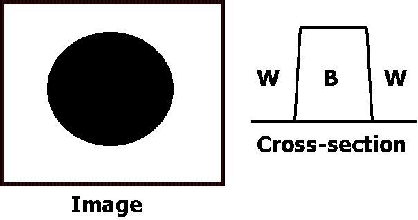
Taking the
absolute value of the derivative results in a waveform with spikes at the
edges. If this is done over the entire image (in two dimensions), it
results in the edge-detected circle.
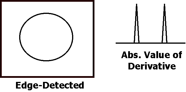
This, however, is
a simplification of the process. What
actually happens is that a 2-dimensional derivative is taken over the
whole image. This is done
using a convolutional kernel.
A convolutional
kernel is a 3 x 3 matrix whose values represent a given operator and that
have some effect on the image they pass over.
To filter an image with a given kernel, the matrix is superimposed
over the image, centered at the pixel of interest.
The pixel values underneath each matrix location are multiplied by
the value in the matrix. The
sum of the multiplicative products is the value for the pixel in the
derived image.
There are
numerous matrix filters that have varying effects on pictures. A well-known one is the mean filter, whose matrix is filled
with 1's. Each pixel is the
average of itself and its closest 8 neighbors, which produces the effect
of blurring an image. The
filters for edge detection are derivative matrix filters.
Although all edge
detection algorithms follow the basic construct of taking two derivatives
and then combining them, the actual values to compute the matrix can be
different. In addition, the
image can be pre- and post-processed to achieve differing results.
Three major edge-detection algorithms were examined
during the course of the project. They
are the Sobel, Prewitt, and Canny operators.
The Prewitt operator was chosen for the project as it had the most
advantageous characteristics. The
following describes the basic properties of the algorithms. A more detailed comparison is done in the next section, Algorithm
Analysis.
Sobel
The Sobel operator is the standard operator used in
many edge detection implementations.
It uses the basic edge detection algorithm with a simple kernel.
Its primary advantages are that it is simple to implement and is
quite fast.
Sobel edges are characterized by thick lines, and the
image sometimes has noisy areas which are points of white against a black
background.
Prewitt
The Prewitt operator is nearly identical to the Sobel
operator. It is as easy to
implement, and just as fast, since the only difference is the set of
values for the convolutional kernel.
However, the Prewitt operator gives a somewhat cleaner image than
the Sobel operator. For this
reason, we chose it as the project's edge-detection algorithm.
Canny
The Canny operator was the most difficult to
implement of the three that were examined.
It employs sophisticated pre- and post-processing techniques, such
as dynamic thresholding, line detection, and thick/thinness filters.
The lines in the edge map are clean, but somewhat anemic since they
are only 1 pixel wide. This is done intentionally, but does not suit the purposes of
this project.
The speed of each
algorithm was measured on a fixed platform (please refer to appendices)
using the Linux ‘time’ command. Each
algorithm was tested on the same 50 frames of video, which was saved on
the hard-drive.
Please refer to the
results section bellow.
All 3 algorithms ran on 50
frames of video. The results are as follows:
Plain viewfinder program:
21.8 secs, framerate was 2.3 frames/sec.
Prewitt and Sobel after
optimization: 27.9 secs,
framerate was 1.7 frames/sec.
Prewitt and Sobel before
optimization: 39.1 secs,
framerate was 1.3 frames/sec.
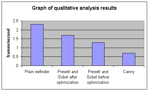
Canny: 66.8 secs, framerate
was 0.7 frames/sec.
As we can see the Sobel and Prewitt algorithms are
almost twice as fast as the Canny when optimized.
The Canny algorithm is slower because it copies the data a few
times into different buffers in order to process the image. Both Sobel and Prewitt algorithms perform the calculations in
one pass.
This covered image clarity
and amount of edge detection analysis on each of the Sobel, Prewitt, and
Canny algorithms.
To eliminate the timing
performance issues from interfering with the results, the algorithms were
first run on 100 frames of video and the edge-detected video was saved to
hard-drive. Then using a
minimal adaptation of the viewfinder program (see appendices) the
edge-detected video was displayed on the monitor for analysis.
This way the results of all 3 algorithms were observed at exactly
the same speed, therefore removing any prejudice regarding the speed of
algorithms.
|
|
Advantages
|
Disadvantages
|
|
Sobel
(Figure in the appendices)
|
Emphasis on important edges like outlines of
objects
Less edge loss than Prewitt (captures more of
the edge detail in the image)
|
Excessive impulse noise obfuscates the image
Edges not as sharp as Canny
|
|
Prewitt
(Figure in the appendecies)
|
Emphasis on important edges like outlines of
objects.
Good sense of depth.
Clean image with no impulse noise.
|
Edges not as sharp as Canny
Some of the important object edges are lost
because of the edge thickness compare with Sobel.
|
|
Canny
(Figure in the appendices)
|
Clean edges
Easier to compress (less noise in image)
Captures sharp edges well
|
Textures interfere with edge detection
obfuscating the important object edges in the image
Picture colors need to be inverted to be more
visible.
Lines are too thin.
All lines have the same thickness which takes
away the sense of depth.
|
The Prewitt algorithm has
been chosen as the perfect fit for this project because of its speed and
the quality of the output video.
The speed of the algorithm
is as fast as Sobel and almost seven times faster than Canny.
Also, being a one-pass algorithm, chances of finding a faster or
more efficient way to perform edge detection is not high.
The Prewitt algorithm also
produces a very clean image that does not have the excessive impulse noise
of Sobel while still producing lines that are very visible.
Because this project is intended to be used by a person suffering
glaucoma or similar vision-reducing illnesses, the output of the image has
to be high-contrast and must have thick and recognizable edges.
The thickness of lines is also very important in providing a sense
of depth and this is one of the reasons an algorithm like Canny can be
impractical.
Optimization was done on the winning algorithm (prewitt),
and was based on the qualitative and quantitative analysis done
previously. Two aspects of
the algorithm could be optimized:
·
Image quality
·
Algorithm speed
These points will be detailed bellow.
Adaptive Dynamic Range Correction
The image from the edge-detection filters can be
further improved by applying some processing.
According to the output desired we could apply different curves
that would map the input pixel value to a predetermined output value.
This way, we can control the quality of the image without modifying
the edge-detection code.
The adaptive dynamic range correction curves are
divided into three families:
·
Stretch curves
·
Binary threshold curve
·
S curves
Each one of these serves a different purpose and are
detailed bellow. Using these
curves, we can construct a large variety of curves that could be used to
improve the image.
Stretch
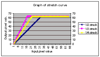 The
values from the digital camera are listed to be between 0 and 63.
However, in actuality, they are between 5 and 25.
This means that some adjusting must be done to make the values
occupy the entire range. This
can be done by a real normalization function, which preserves the standard
deviation of the values while shifting the mean to 32.
However, a function like this would be too costly for our real-time
system. The next best thing
is to use a stretch curve, which performs a simple linear shift of values. The
values from the digital camera are listed to be between 0 and 63.
However, in actuality, they are between 5 and 25.
This means that some adjusting must be done to make the values
occupy the entire range. This
can be done by a real normalization function, which preserves the standard
deviation of the values while shifting the mean to 32.
However, a function like this would be too costly for our real-time
system. The next best thing
is to use a stretch curve, which performs a simple linear shift of values.
The stretch curve is usually combined with other
curves that improve the image further.
Binary Threshold
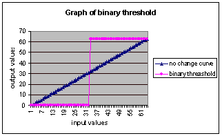 The
pixels can be mapped to minimum value, 0, or maximum value, 63.
This is called a binary threshold and is used ‘clean up’ the
image. By setting the
threshold value we can obtain different ouputs.
If the image is already corrected with a stretch curve, 50% mark
would be a good start value for the threshold.
This w ay any value larger than 32 would be mapped to 63 and all
others map to 0. The
pixels can be mapped to minimum value, 0, or maximum value, 63.
This is called a binary threshold and is used ‘clean up’ the
image. By setting the
threshold value we can obtain different ouputs.
If the image is already corrected with a stretch curve, 50% mark
would be a good start value for the threshold.
This w ay any value larger than 32 would be mapped to 63 and all
others map to 0.
The binary threshold causes the image to lose some
data. This is because the
mappings are none reversible. This
loss translates to a lack of sense of depth in the image with is not
desired. Therefore, we need
‘softer’ transformations using S curves.
S Curves
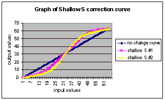
S curves are divided into two different groups:
·
deep S curves
·
shallow S curves
 |
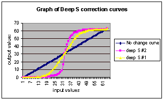 |
Deep curves change the middle section of the range by
mapping the values more towards the extremes, while shallow curves perform
a softer but mo re global transformation.
The effect of an S curve is similar to adjusting the brightness and
contrast levels of the output video.
This could give a very pleasing result, by making the image more
visible with out visible loss of information.
The sense of depth is preserved while the image looks brighter.
The perceived resolution of the image is also higher than that of
binary thr eshold because of the softer change around edges. A sharp pixel value change results in jagged edges, which
gives the impression of low resolution.
To speed up the algorithms we looked tried to locate
the places in the programs where optimization could help. The most important issue is the input frame rate.
With our video camera (quickcam), we received video at just under 3
frames per second. With the
addition of the viewfinder code, the frame rate dropped down to 2.3
frames/sec. At this speed, we
do not have video but a sequence of images that have an effect similar to
slow motion. Since all out
algorithms use the viewfinder program, 2.3 frames/sec results in an upper
limit for optimization.
Besides the input frame rate, the actual algorithms
were optimized in the following way:
Integer Calculation
The edge detection code includes pixel calculations
which are usually performed as floating point operations. This is a problem with Pentium based computers because the
Pentium chip works much slower with floating point values than with
integer ones. By using an
integer approximation anytime there is a floating point value (casting to
int in C programming language), we can improve the speed of the
algorithms. This is possible
because for our programs, the error resulting from quantization to integer
values is not visible to the user.
Lookup Tables
The major cost in the edge detection algorithm is a
Pythagorean calculation of two values.
The format of this calculation is the following:
Result = sqrt( sqr(value1) / 2 + sqr(value2) / 2 )
Since we know the range of input values, we can do
all the calculations beforehand and record them in a two dimensional
array. At runtime, all we
have to do is to look up the already calculated value.
The cost of a lookup is minimal whereas the cost of performing the
calculation for each pixel is major.
Without this optimization, the program runs 3 times faster.
The lookup table code is included in the filters.c program in the
appendix. Here is the heart
of the function:
lookup[i][j] = (char) ((int) sqrt(i*i/2 + j*j/2) );
where i and j are value1 and value2 respectively and
lookup is the lookup array.
No Multiplications or Divisions
The cost of multiplication is much larger than that
of addition when done in computer’s CPU.
For this reason, we replaced all runtime multiplications with
additions which improved the speed of the operation considerably.
This was only possible since the never had to multiply by more than
2. Division also provides the
same problem. Luckily, when
performing division by 2, we can shift the binary version of the number by
one to the right. The cost of
this is much less than that of division. This of course is not possible when dividing by values that
are not power of 2. |


